Custom signals

Plot a quantity the controller does not publish, as an arithmetic expression over signals that it does.

7 minute read

A custom signal is a trace whose value is an expression over other signals: a tracking error where the controller publishes only actual and target, a magnitude built from components, a unit conversion, or a constant reference line. It is computed in the browser and drawn like any other trace.

Note

Plot the controller’s own parameter first whenever there is one. A computed copy of a value the controller already publishes starts empty, is only as fast as the subscription, and can drift from the number the controller actually uses.

Your first custom signal

A six-axis robot publishes jointPositionsActual and jointPositionsTarget but no per-joint error. This builds that error, in degrees, for all six joints at once. You need a connected controller.

Click + Custom signal above the tree in the Active panel.
Name it jointError. The signal lives at formulas/jointError, a sibling of root/, so it can never be mistaken for a controller path.
Write the expression:
```
deg(${root/ManipulatorControl/jointPositionsActual} - ${root/ManipulatorControl/jointPositionsTarget})
```
You do not have to type those paths. While the editor is open both signal trees become a palette: a plain click in the Parameters tree or the Active list inserts a reference at the caret instead of doing its usual job. Clicking an array’s name inserts the whole array; clicking a chN row inserts just that element.
Press Enter. Six traces appear under formulas/jointError, one per joint: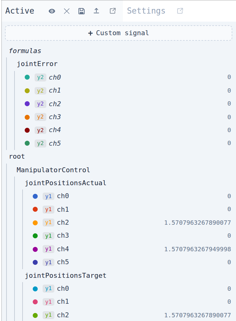

What Desk did with that

Three things happened that are worth knowing before you write a second one:

It fanned out. Neither reference carried an index, so the formula was evaluated element by element: one trace per joint, each with its own colour, axis and visibility. See the Arrays tab.
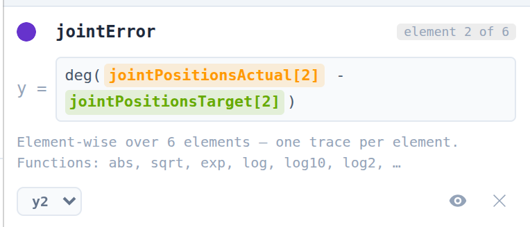
It subscribed the inputs. jointPositionsActual and jointPositionsTarget were added hidden, so the formula has data without drawing lines you did not ask for. See the Lifecycle tab.
It kept the expression readable. Select any channel and the details pane renders the formula as chips, each reference in the colour of the trace it reads and resolved to the element you are looking at: [2], not the abstract shared form:

A committed expression rendered as coloured chips, resolved to element 2

Expression reference

Start with Syntax; the rest are independent and can be read in any order.

Referring to a signal

Every reference to another signal is wrapped in ${…}:

Written	Reads
`${root/ManipulatorControl/jointTorquesActual}`	That parameter
`${root/ManipulatorControl/jointTorquesActual[0]}`	One element of an array parameter
`${x}`	The plot’s X axis: seconds since the time origin, or the X-source signal in XY mode

${t} and ${time} are accepted for the X axis as well, and all three spellings collapse to one reference.

A leading y = is stripped, so y = ${root/a} * 2 and ${root/a} * 2 are the same expression.

Operators

+ - * / % ^, parentheses, and unary sign.

Unary minus binds looser than ^, so -${a}^2 is −(a²), as in ordinary mathematical notation. Write (-${a})^2 if you meant to square the negated value.

When an expression will not compile

It is never stored. The editor stays open with the parser’s message, so the plot never carries a trace that silently produces nothing.

Functions

abs sqrt exp log log10 log2 sin cos tan asin acos atan sinh cosh tanh floor ceil round sign atan2 pow hypot min max clamp

min and max are variadic and pure: they compare their arguments at the current sample and nothing else. So max(${root/a}, 0) clamps a signal at zero. For the rolling versions see the Windows tab.

Angles

The controller works in radians; you usually want to read degrees.

Written	Value
`deg(v)`	Converts radians to degrees
`rad(v)`	Converts degrees to radians

A joint error is far easier to judge in degrees, which is why the worked example wraps the subtraction in deg(…).

Constants

pi, e, tau.

A constant on its own is a valid expression, so 0.5 draws a horizontal reference line at 0.5, handy for marking a tolerance band against a live signal.

These functions read a trailing time window rather than only the current sample. All of them are spelled (signal, seconds):

Function	Value
`average(v, s)`	Rolling mean over the last s seconds. The usual way to make a noisy error readable. `avg` is accepted too
`movmax(v, s)` / `movmin(v, s)`	The extreme over the window. `maximum` and `minimum` are accepted too
`rate(v, s)`	Change per second across the window. A derivative whose window length is also its smoothing

Two worked lines

Smooth a noisy torque signal over two seconds:

average(${root/ManipulatorControl/jointTorquesActual[0]}, 2)

Peak-to-peak of the same signal over five seconds:

movmax(${root/ManipulatorControl/jointTorquesActual[0]}, 5) - movmin(${root/ManipulatorControl/jointTorquesActual[0]}, 5)

The rolling functions take the signal-processing spelling rather than overloading min and max, because a rolling minimum and a two-argument minimum cannot be told apart by their arguments.

How the window behaves

It answers from the very first sample rather than leaving the trace blank while the window fills, so a fresh average is simply a mean over fewer points at first.
It is measured against controller time, not against the X axis, so it keeps its meaning in XY mode.
Each call site keeps its own history. That history restarts when you edit the expression, when the session reconnects, or when time runs backwards. A window never blends two timelines.

A reference with no index reads the whole parameter, and the formula is then evaluated element by element: element i of the result is computed from element i of every array input. This is what turns the worked example’s single expression into one trace per joint.

Each element gets its own colour, axis and visibility, exactly like the channels of an ordinary array parameter.

Mixing widths

Two kinds of reference broadcast, giving the same number to every element:

a scalar parameter, ${root/Logic/mode};
an indexed reference, ${…/jointPositionsTarget[0]}, which always reads element 0 whatever element of the formula it is feeding.

So this subtracts joint 0’s target from every joint’s actual:

${root/ManipulatorControl/jointPositionsActual} - ${root/ManipulatorControl/jointPositionsTarget[0]}

The formula’s width is the widest unindexed array it reads. Combining arrays of different widths is allowed, but the elements past the end of the shorter one have no value to read and simply produce no sample, so those traces stay empty. Index the shorter array if you meant to broadcast it.

Width is re-derived, not fixed

The width comes from the parameter tree whenever the tree can answer. A formula written while disconnected therefore fans out on connect, and collapses back to a single trace if you edit the expression so it no longer reads an array.

One formula, one signal

Removing any single element removes the whole formula. From your side it is one signal, and a partial one would immediately be rebuilt.

Inputs are subscribed for you

A signal a formula reads that is not already plotted is added hidden: it subscribes normally so the formula has data, takes a palette colour, and shows a live value, without drawing a line you did not ask for.

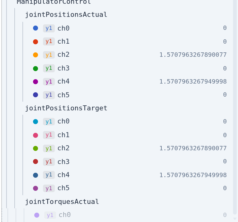
An auto-added input listed dimmed below the plotted traces

Plotting one by hand promotes it to an ordinary visible trace, and it then survives the formula that pulled it in. Inputs that no formula still references are dropped again.

Validation

References are checked against the live parameter tree when you commit. An unknown path, a non-numeric parameter or a channel outside the array is refused, with every problem named at once rather than one per attempt.

The check is skipped while disconnected, where there is nothing to check against, which is why a formula written offline can still be saved, and is validated on the next connect.

Saving and restoring

Custom signals and their auto-added inputs are written to traces.json along with the ordinary traces, so a saved setup restores them. See Plotting.

Formulas with no live input

A formula that reads no controller signal (a bare constant, or one reading only ${x}) has no publish cycle to ride on, so it is driven by a local 30 Hz clock instead. sin(${x}) therefore draws with no controller connected at all, which makes it a quick way to check that a plot is alive.