Plotting

Add signals to the plot and manage them in the Active panel.

8 minute read

Each plotted signal is a trace. Desk draws them with a WebGL renderer, so hundreds of thousands of points per trace stay interactive.

Joint positions and torques on two Y axes

Your first traces

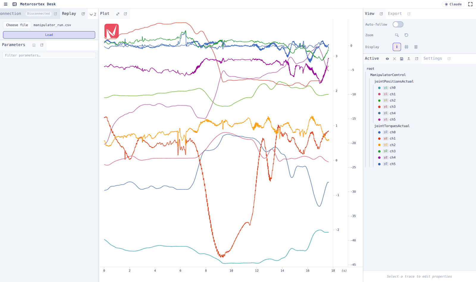
Plotting a six-axis robot’s joint positions against its joint torques, which is the commonest thing you will do and the one that teaches the one habit that matters: one axis per unit.

In Parameters, type jointPositionsActual in the filter box.
Double-click the parameter itself, not a channel. All six channels arrive at once, on axis y1, each with its own colour.
Filter for jointTorquesActual and double-click that too. Six more traces, but they also land on y1, and newton-metres against radians means the torques flatten the positions into a line.
In Active, click the jointTorquesActual folder row. All six of its channels select together.
In the details pane at the bottom, set the axis dropdown to y2.

The torques move to their own auto-scaled axis on the right, and both groups are readable at once. That is the rule in general: signals sharing a unit share an axis, a different unit gets its own.

Note

Nothing here writes to the machine. Adding a trace only subscribes to a parameter, so you can plot as freely as you like.

Reference

Adding first; the rest stand alone.

From the Parameters tree:

Action	Result
Double-click a numeric leaf	Add it as a trace (double-click again to remove)
Double-click an array parameter	Add all its channels at once (again removes them all)
Expand an array, then double-click a channel	Add a single channel
Right-click → Add to plot / Delete from plot	Same as double-click

New traces land on axis y1 and take the next colour from the palette.

Non-numeric parameters (strings, enums, byte arrays) can be read in the tree but not plotted.

When the controller does not publish what you want

A tracking error, a magnitude, a unit conversion: write it as an expression instead, with + Custom signal above the Active tree. See Custom signals.

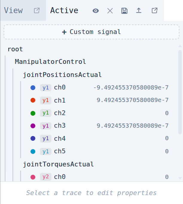
Active panel with the signal tree and the details pane

Active lists everything currently plotted as a tree that mirrors the parameter paths, so twelve channels of two parameters read as two groups rather than twelve long paths. Every row shows the trace colour, its axis badge (y1…y4 or x) and the live value. A row whose signal is a writable controller parameter also carries its own input, so its value can be changed without selecting it first.

Hidden traces are greyed out; the x-source row is marked separately.

Selecting signals

Selecting traces emphasises them three ways at once: they are drawn thicker on the plot, their names are bolded in the legend, and their lines are lifted in front of the others. That is what makes one signal findable in a crowded plot.

Gesture	Selection
Click	Select this signal. Clicking the only selected signal again clears the selection
Click a folder row	Select every signal under it
Ctrl / Cmd + click	Add or remove one signal (or a whole folder)
Shift + click	Select the range between the last click and this one
Click empty space	Clear the selection

The selection also drives the arrow, H and Del keys, and it is what the Statistics panel reports on. See Keybindings.

Picking a trace off the plot

The plot answers the other way round too. Hover a trace and the pointer becomes a hand, and a small card names the parameter as path[channel], outlined in that trace’s own colour. It is the quickest way to identify a line without reading down the list.

Click it and the matching row is selected in Active, bringing the panel forward if it sits behind another tab. A trace counts as hovered when its nearest sample is within fifteen pixels of the pointer; a click that lands on nothing leaves the selection as it was.

Hover and picking stand down while you are capturing a measurement, so measuring still gets its clicks.

Panel header buttons

Button	Action
Eye	Hide all traces / show all traces
✕	Remove all traces
Save	Save the trace list to a `traces.json` file
Load	Add the traces from a `traces.json` file to the ones already plotted

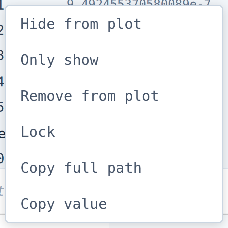
Right-click a row for:

Item	Action
Hide from plot / Show on plot	Stop or resume drawing it, leaving it subscribed
Only show	Hide every other trace, so this one stands alone
Remove from plot	Drop it
Lock / Unlock	Force the parameter at its current value, or release it
Copy full path	Copy the `root/…` path to the clipboard
Copy value	Copy the current value

On a folder row the action applies to every signal underneath it, and the labels say so: Hide all from plot, Only show these, Remove all from plot. Lock appears only for a single writable controller parameter, so not on folders, custom signals, or a path the tree does not know. Copy value is a leaf action only.

The same menu is available on the rows of the plot legend.

The pane at the bottom of Active acts on whatever is selected.

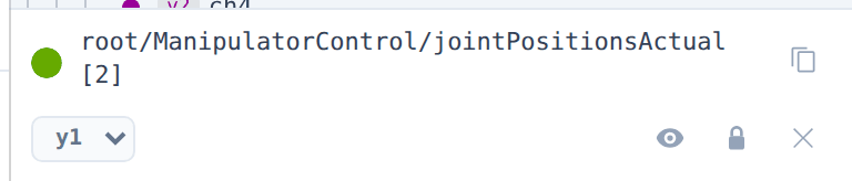
Control	What it does
Colour swatch	Pick the trace colour
Path	Full path with channel index; the copy button copies it
Value input	Write a value to this parameter (math expressions allowed, Enter to apply)
Axis dropdown	Move the trace to `y1`–`y4`, or make it the `x` source
Eye	Hide or show the trace
Lock	Force the parameter at a value, or release it
✕	Remove the trace

A writable signal also carries a write input on its own row in the list, so a quick change does not need the row selected first. Both write the same way.

Acting on several traces at once

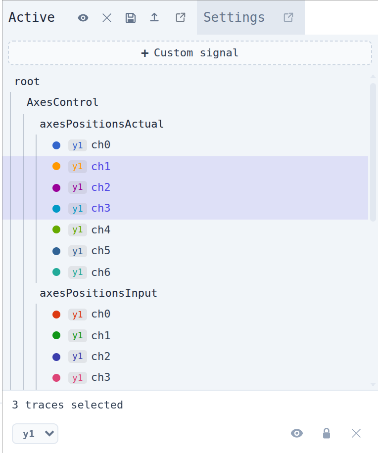
With more than one signal selected the pane shows N traces selected and applies the axis, hide, lock and remove actions to all of them together, which is how you move a whole parameter’s channels to another axis in one go.

What hiding actually does

A hidden trace stays subscribed. It keeps receiving data and can be revealed later without a gap in its history, but it is not drawn, and it is left out of CSV export.

Use it to park a signal you want to keep recording but not look at.

Four Y axes

Each trace sits on one of four independent Y axes, y1–y4. An axis appears as soon as a trace is assigned to it and disappears when its last trace is removed, and each one auto-scales to the traces on it.

Group traces by physical unit: signals sharing a unit belong on the same axis, and a different unit or a very different magnitude belongs on another. Otherwise the larger signal squashes the smaller one flat.

Keep an actual and its target on the same axis, though: they share a unit, and overlaying them is the whole point of plotting them together.

Tip

A six-element pose is two units in one parameter: elements 0-2 are metres and 3-5 are radians. Add those channel by channel onto two axes rather than adding the whole array at once.

XY mode

Set a trace’s axis to x and the plot switches from time to XY: that signal becomes the horizontal axis and every other trace is drawn against it: actual versus commanded position, or a tool path in a plane.

The x-source trace itself is not drawn, so it has no colour and no eye button. Only one signal can be the x source, and it has to be a single channel rather than a whole array.

Set its axis back to y1–y4 to return to time mode.

Save in the Active panel header writes the current signals to a traces.json file: path, channel, colour, axis and hidden flag for each, plus any custom signals and the inputs they pulled in.

The browser’s own Save dialog opens so the file lands next to the run it describes rather than under one fixed name in the download folder. The set is copied to the clipboard as well, ready to paste into an issue or a message.

Loading adds, it does not replace

Load adds the file’s traces to whatever is already plotted and resubscribes them. Signals already on screen are left alone: they keep their colour and axis, and the file does not restyle them.

That makes a saved set a building block: two of them together, or one on top of what you are watching now. To start from nothing instead, click ✕ (remove all) first.

Paths that are not on this controller

What happens depends on whether there is a controller to ask:

Connected: paths that do not exist here are dropped as the file loads.
Disconnected: everything is kept, and pruned at the next connect.

So a trace set built against one machine can be loaded offline and will sort itself out when you reach a controller that has those signals.